Remote Sensing Lab #8: Spectral Signature Analysis

Goals and Background

The main objective of this lab is to understand how to obtain and interpret spectral reflectance signatures from various Earth surfaces captured by satellite images.  To perform the objective I will be using Erdas Imagine 2015 to collect, graph, and analyze spectral signatures to determine if they pass the spectral separability test.

Methods

I was provided a satellite image from the year 2000 of the Eau Claire and Chippewa Falls area in Wisconsin.  I was instructed to collect spectral signatures from the following list of Earth and near surface materials.

1.  Standing Water
2.  Moving Water
3.  Vegetation
4.  Riparian Vegetation
5.  Crops
6.  Urban Grass
7.  Dry Soil (uncultivated)
8.  Moist Soil (uncultivated)
9.  Rock
10.  Asphalt Highway
11.  Airport Runway
12.  Concrete Surface (Parking lot)

To obtain the spectral signatures in Erdas I will be utilizing the Polygon tool under the Drawing tab (Fig.1).  After drawing an outline of the area of interest (AOI) to collect the spectral signature from, I opened the Signature Editor from the Supervised menu in the Raster tab of Erdas.  With the Signature Editor open I used the Create New Signature from AOI and Display Mean Plot Window to add the signature from the polygon to the window and display the graph of the spectral signature (Fig. 2).

(Fig. 1) Polygon tool (highlighted in yellow below Manage Data) found in the Drawing tab.

(Fig. 2) AOI outline (center,with blue nodes surrounding), Signature Editor (left) and the Signature Mean Plot graph (right)

I proceeded to repeat this process for the entire list I was given.  In the Signature Editor I was able to change the Signature Name (label) for each of the spectral signatures, which transferred to the graph as well.  The majority of the surface materials were easy to identify from the given image.  Utilizing the Google Earth Link/Sync feature with in Erdas helped me to identify surface features which were not easily identifiable.

Analyzing the spectral signatures is the next step.  Selecting two of the signature at the same time in the editor window and then selecting Multipule Signature Mode on the plot window allows you to view more than one signature (Fig. 3).

(Fig. 3) Two signatures selected and displayed in the plot graph.

Results


Analyzing the graph of reflectance from (Fig. 3) we are able to see the variation between standing water and moving water.  The variation displayed between the two water surfaces is explained through Specular and Diffuse reflection.  The movement and ripples in the moving water give it diffuse reflection which send the reflections in all directions and reduces the intensity.  Where as the standing water is smooth has a more specular reflection, which sends the reflectance back with a higher intensity.  Multiple variations of this type of analysis can be done from the spectral information gathered in this manner.  

(Fig. 4) Final graph will all 12 surface spectral signatures plotted.

Sources

Satellite image is from Earth Resources Observation and Science Center, United States
Geological Survey.

Remote Sensing Lab #7: Photgrammetry

Goals and Background

The objective of this lab is to learn how to perform photogrammetric tasks on satellite image and aerial photographs.  The beginning portion of the lab is designed to help me understand the mathematics behind the calculations which take place in photogrammetric tasks.  The later portion of the lab will give me and introduction to stereoscopy and performing orthorectification on satellite images.  The completion of this lab will give me the basic tools and knowledge to perform multiple photogrammetric tasks.

Methods

Scales, Measurements, and Relief Displacement
 
The first portion of this lab I will be completing multiple measurements and calculations on aerial photographs.  I will be utilizing Erdas Imagine for one of the calculations and manual calculating the other measurements. 

Calculating Scale of Nearly Vertical Aerial Photographs

The ability to calculate the scale of a aerial photograph is an essential which everyone in the remote sensing field must have the ability to do.  Calculating the scale can be done in a couple different manners.

One of the ways to complete this calculation is to take a measurement of two points on your aerial photograph and compare that measurement to the real world distance.  Though this is a great and simple method it isn't always possible to obtain a measurement in the real world.  I will discuss the method to be used when real world measurements are not possible a little later.

Utilizing an image and labeled by my professor I measured from point A to point B with my ruler and got a measurement of 2.7 inches. (Fig. 1).  I was give the dimension in the real world from point A to point B was 8822.47 ft.  My next step I converted the real world dimension to inches which was 105869.64.  This left me with a fraction of 2.7/105869.64.  The last calculation was to divide the numerator and the denominator by 2.7 which gave me an answer of 1/39210.  I was instructed to round to the nearest thousand for my answer.  The scale of this aerial image is 1/40,000.

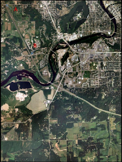
(Fig. 1)  Image with label points to calculate measurements from (Not calculated at the scale the image is displayed)

Photographic scale can be calculated without a true real world measurement as long as you know the focal length of the camera and the flying height above the terrain of the aircraft which took the image.  We were given all of the information need to calculate the scale of a different image (Fig. 2) from our professor.  The information I was given was as follows: Aircraft altitude= 20,000 ft, Focal length of camera=152 mm, and the elevation of the area in the photograph=769 ft.

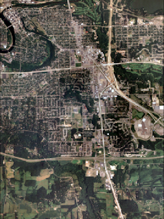
(Fig. 2) Image I calculated scale for utilizing the camera and altitude dimensions.

The first step was to convert all of the data information in to the same measurements. To reduce the risk of conversion errors I decided to convert the focal length which was the only measurement that wasn't in feet.  Converting 152 mm to feet gave me a dimension of .4986816 ft.

Using the formula Scale= f/H-h with the dimensions showing the the image below (Fig. 3). you are able to calculate the scale of the image.  Using the formula I input the numbers I was given: .4986816/(20000-796).  Completing the math in the denominator gave me a fraction of .4986816/19204.  Dividing the numerator and denominator by .4986816 gave me a fraction of 1/38509.  Rounding the denominator to the nearest even thousand gave me a fraction representing the scale of the image of 1/40,000.

(Fig 3.) Detailed description and display of measurements required to calculate image scale.

Measurement of areas of features on aerial photographs

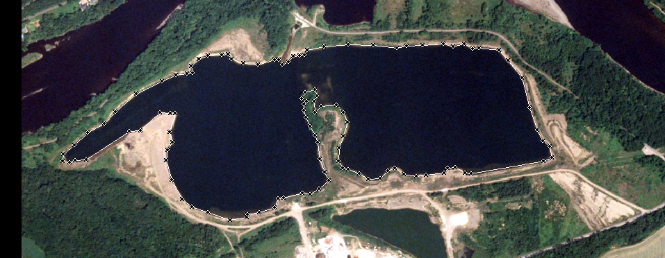
For this section of the assignment I will be utilizing Erdas Imagine to calculate the area of a lagoon in an aerial image (Fig. 4) given to me by my professor.

Utilizing the polygon measurement tool in the measure tool bar (Fig. 4) I traced the outline of the lagoon to be able to calculate the perimeter and area (Fig. 5).

(Fig. 4) Measure tool bar with the polygon tool selected.

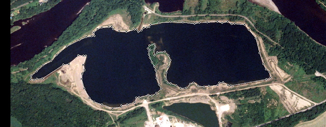
(Fig. 5) Outline using the measurement tool in Erdas Imagine.

Once the polygon has been completed the measurement are displayed in the Measurements window (Fig. 6).  Utilizing the tool bar at the top you can alter the measurements to into multiple varieties such and inches, feet, meters (Perimeter) and acres, square feet, or square meters just to name a few.

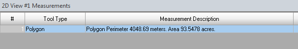
(Fig. 6) Perimeter and Area displayed in the Measurement window.

Calculating relief displacement from object height

Relief displacement is the variation of objects and features within an aerial image from their true planimetric position on the ground.  Looking at (Fig. 6) you will see a smoke stack label "A".  You can see the smoke stack is at an angle.  In the real world if you were standing next to the stack it would be perfectly vertical and not leaning or at an angle.  This "displacement" related to the location of the Principal Point (center of the image when it was taken) and the location of the feature.  The scale of the image is 1:3209 and the camera height is 3,980 ft.

To calculate the relief displacement (d) you must know the height of the object in the real world (h), radial distance from the principal point to the top of the displaced object (r), and the height of the camera when the image was taken (H).  To calculate the displacement you use the formula (D)isplacement= h*r/H. 

To complete the forumla I needed to obtain 2 different variables which were not provided for me.  I need to calculate the heights of the smoke stack using the scale and I needed to measure the distance from the principal point to the top of the smoke stack.  Using the scale and a ruler I determined the height of the smoke stack was 1604.5 inches and the radial distance from the principal point was 10.5 inches.  I converted the camera height to feet which gave me 47760 inches.  Inputting these variables into the formula gave me the displacement of .352748 inches.  To correct this image the smoke stack would have to be pushed back the .352748 inches to make vertical.

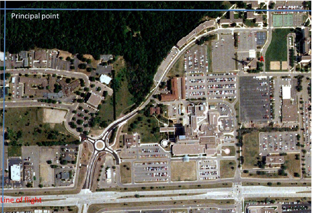
(Fig. 6) Image to calculate relief displacement from.

Stereoscopy

Stereoscopy is the science of dpeth perception utilizing your eyes or other tools to view a 2 dimensional (2D) image in 3 dimensions (3D).  You can use multiple tools such as a Stereoscope, Anaglyph and Polaroid glasses, or through development of a stereomodel to view 2D images in 3D.

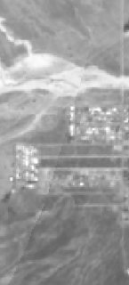
In this lab we will be utilizing Erdas Imagine to create an Anaglyph.  To create the Anaglyph we will be using Anaglyph tool with in the Terrain menu tab.  I imported an aerial image and a Digital Elevation Model (DEM) (Fig. 7) of the same area into the Anaglyph Generation menu.  Then  next step is to run the tool, and after it is complete you can open up the Anaglyph image in Erdas.  Once open in Erdas or any other image viewing tool you can use Polaroid glasses (3D glasses) to view the image in 3D (Fig. 8).

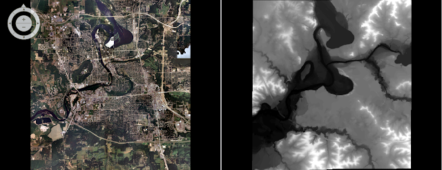
(Fig. 7) Aerial image (left) and DEM (right) used to create Anaglyph in Erdas Imagine.

(Fig. 8) Anaglyph image produced in Erdas Image, if you use Polaroid glasses you will be able to see the image in 3D.

Orthorectification

Orthorectification refers to simultaneously removes positional and elevation errors from one or multiple aerial photographs or satellite images.  This process requires the analyst to obtain real world x,y, and z coordinates of pixels on aerial images and photographs.  Orthorectified images can be utilized to create many products such as DEM's, and Stereopairs.

For this section of the lab I will be using Erdas Imagine Lecia Photogrammetric Suite (LPS).  This tool with in Erdas Imagine is used for triangulation, orthorectification with digital photogrammetry collected by varying sensors.  Additionally, it can be used to extract digital surface and elevation models.  I will be using a modified version of Erdas Imagine LPS user guide to orthorectify images and in the process create a planimetrically true orthoimage.

I was provide two images which needed orthorectification.  The images overlapped a specific area but but were not exactly the same.  When you brough them into Erdas they layed perfectly on top of one another.  For this reason I knew the images needs to be corrected.

The first step was to create a New Block File in the Imagine Photogrammetry Project Manager window.  In the Model Setup dialog window I set the Geometric Model Category to Plynomial-based Pushbroom and selected SPOT Pushbroom in the second section window.  In the Block Property Setup I set the projection to UTM, the Spheroid Name to Clarke 1866, and the Datum to NAD 27 (CONUS).  I then brought in the first image and verified the the parameters of the SPOT pushbroom sensor in the Show and Edit Frame Properties menu.

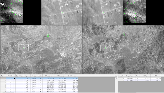
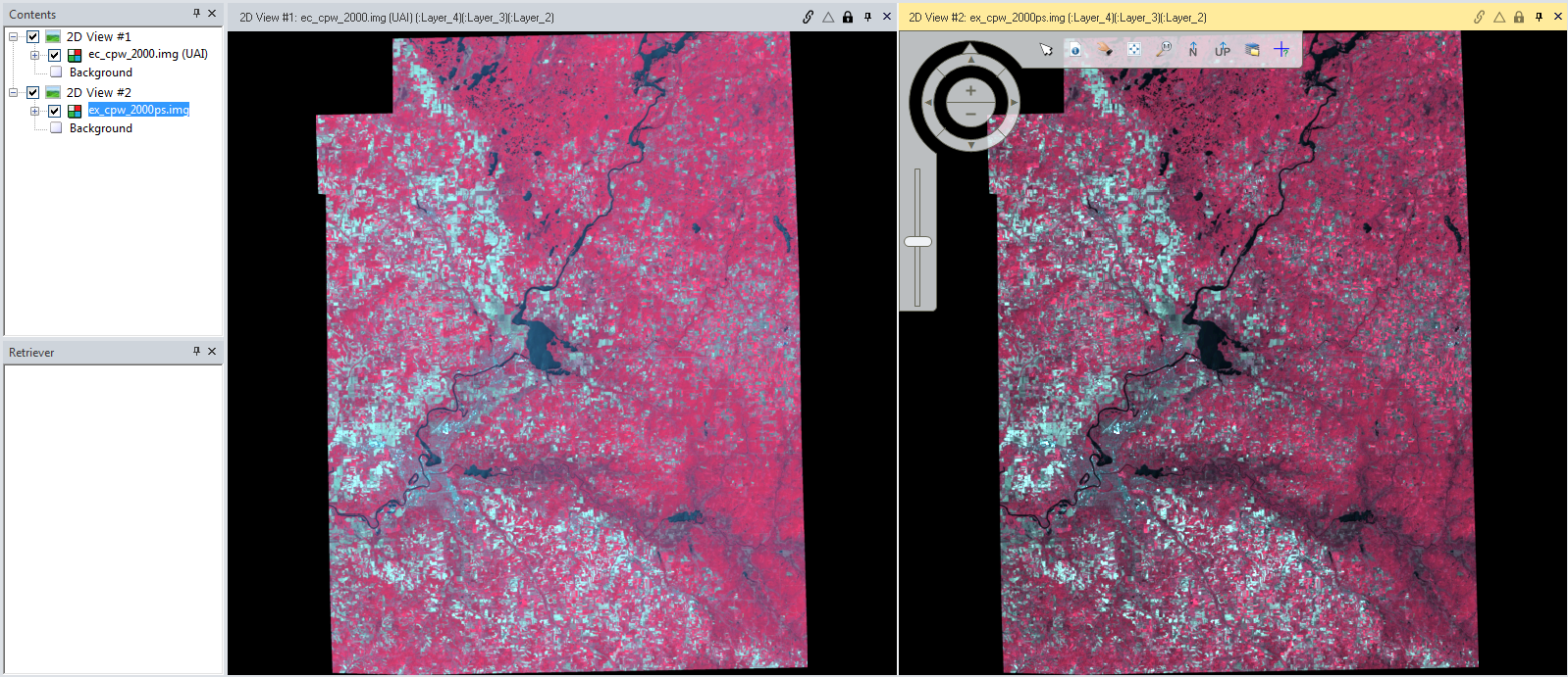
The next step I activated the point measurement tool and started to collect GCP's.  I set the point measurement tool to Classic Point Measurement Tool.  Using the Reset Horizontal Reference icon I set the GCP Reference Source to Image Layer.  I was then prompted to import the reference image, and checked the Use Viewer AS Reference box.  Now I had one of the images which needed to be corrected in the viewer with a reference image which had  been previously corrected (Fig. 9).  I was given the location for the GCP from my professor.  I proceeded to locate 9 GCP's on the uncorrected image and the reference image.  Utilizing the same method I collected 2 other GCP's from an alternate image.

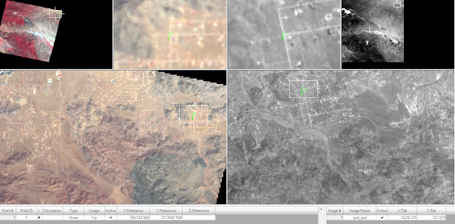
(Fig. 9) Collecting GCP's with the reference image (left) and the uncorrected image (right).

The next step was to set the Vertical Reference Source and collect elecation information utilizing a DEM.  Clicking on the Reset Vertical Reference Source icon opens a menu to set the Vertical Reference Source to a selected DEM.  After selecting the DEM in the menu I selected all of the values in the cell array and clicked Update Z Values on Selected Points icon.  This set the Z (elevation values) to the GCP points I had previously set.

After all of the GCP's were added and the elevation was set to the first image I needed to import the second image for correction.  To properly complete this step I had to set the Type and Usage for each of the control points.  I changed the Type to Full and the Usage to Control for each of the GCP's.

Now I was able to use the Add Frame icon and add the second image for orthorectification.  I set the parameters and verified the SPOT Sensor specifications the same as the first image.  With both images brought into the viewer I was able to click on one of the GCP's from the list and then add a GCP to the second image to reference the locations between the 2 images (Fig. 10).  I correlated GCP's for points 1,2,5,6,8,9,and 12 (technically 11).

(Fig. 10) Original GCP selected (blue highlighted lower left) and selected corresponding area in second image for correction.

Next I used the Automatic Tie Point Generation Properties icon to calculate tie points between the two images.  Tie points are points which have an unknown ground coordinates but are able to be visually identified in the overlap area of images.  The coordinates of the tie points are calculated during a process called block triangulation.  Block triangulation requires a minimum of 9 tie points to process.

In the Automatic Tie Point Generation Properties window I set the Image used to All Available and the Initial Type to Exterior/Header/GCP.  Under the distribution tab I set the Intended Number of Points/Images to 40.  After running the tool I was able to inspect the Auto Tie Summary to inspect the accuracy.  The accuracy was good for the points I inspected so I made not changes.

Next I ran the Triangulation tool after setting the parameters as follows.  Iterations wtih Relaxation was set to a value of 3, Image Coordinate Units for Report was set to Pixels.  Under the Point tab I set the type to Same as Weighted Values and the X,Y, and Z values to 15 to assure the GCP's are accurate with in 15 meters.  After running the tool a report was displayed to asses the accuracy (Fig. 11).  In the report our able to examine a number of parameters including the RMSE.

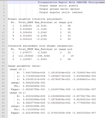
(Fig. 11) Triangulation Report from Erdas Imagine.

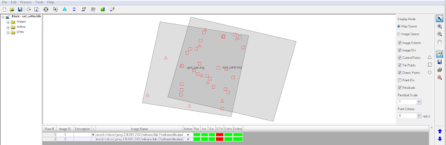
(Fig. 12) Project Manager window display after triangulation was completed.  This shows how the images are overlapped.

The final step of this lab was to run the Ortho Resampling Process.  Making sure I had the first image selected in the project management screen, I used the DEM I used previously, and set the Resampling Method to Bilinear Interpolation under the Advanced tab.  Next I added the second image through the Add Single Output window.  Once the tool was ran I had completed the task of Orthorectification of these two images.

Results







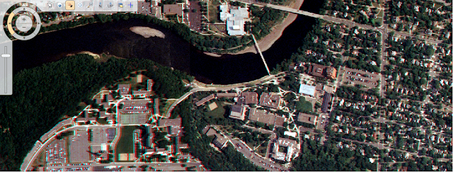
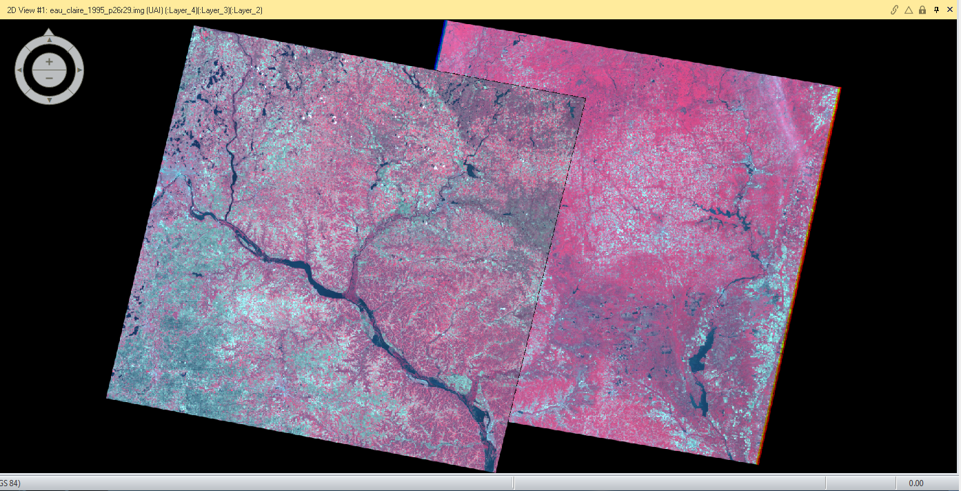
The final results of my Orthorectification resulted in accurately positioned images (Fig. 13).  When zoomed in you can not tell beside the color variation where one picture ends and the other one begins (Fig. 14).

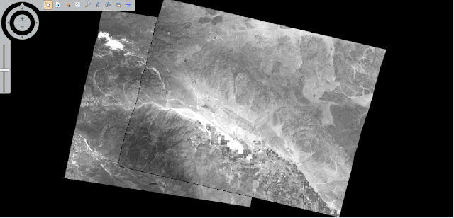
(Fig. 13) Final product of the two images after Orthorectification.

(Fig. 14)  Zoomed in image along the transition from one image to the next.

Data Sources

National Agriculture Imagery Program (NAIP) images are from United States Department of
Agriculture, 2005.
Digital Elevation Model (DEM) for Eau Claire, WI is from United States Department of
Agriculture Natural Resources Conservation Service, 2010.
Spot satellite images are from Erdas Imagine, 2009.
Digital elevation model (DEM) for Palm Spring, CA is from Erdas Imagine, 2009.
National Aerial Photography Program (NAPP) 2 meter images are from Erdas Imagine, 2009.

Remote Sensing Lab #6: Geometric correction

Goals and Background

The goal of this lab is to give us an introduction to a preprocessing method called geometric correction.  Geometric correction is required to properly align and locate an aerial image.  Aerial images are never perfectly inline due to a multitude of factors which alter the angles of the image.  Within this lab exercise we will explore and practice two different methods of geometric correction.

Rectification is the process of converting a data file coordinate to a different coordinate or grid style system known as a reference system.

1. Image-to-Map Rectification:  This form of geometric correction utilizes a map coordinate system to rectify/transform the image data pixel coordinates.

2. Image-to-Image Rectification:  This form of gemteric correction uses a previously corrected image of the same location to rectify/transform the image data pixel coordinates.

Methods

The first method I explored in the lab was Image-to-Map-Rectification.  For this exercise we used a USGS 7.5 minute digital raster graphic (DRG) covering a portion of Chicago, Illinois to geometrically correct a Landsat TM image of the same area (Fig.1).  I will be performing this task in Erdas Imagine 2015.

(Fig. 1) The USGS DRG is on the left and the uncorrected image of Chicago area is on the right

I will be utilizing the Control Points option under the Multispectral tab in Erdas to perform the geometric correction.  After opening the Control Points option I set the Geometric Model to Polynomial and used the first order polynomial equation per directions from my professor.  I also set the USGS DRG map as the reference image.

To correct the image I will be placing ground control points (GCP) on both maps in the same locations using the "Create GCP" tool within the correction window.  At this extent in (Fig. 1) it is hard to be super precise when placing GCP's so after they are placed you can zoom in and adjust them to have a more precise location.  When placing GCP's you want to use fixed locations like "T" intersections of roadways or permanent buildings which have been in the area for a long time.  It is not advisable to used features such as lakes or rivers as they change over time and their locations may be different from image to image.  The accuracy between my GCP points is automatically calculated by Erdas in Root Mean Square (RMS) error.  The industry standard in remote sensing is .5 RMS error or below.  For this first exercise I was only required to reach an RMS error of 2 since this was my first attempt of geometric correction.

I place four GCP's per my instructions in the general area requested by my professor (Fig. 2).  I zoomed in and continued to adjust the points till I was able to achieve a .2148 RMS error, well below the industry standard.  There was very minimal error in the image we corrected, so displaying the correction is very difficult.  In the next correction process you will be able to see and visible change from the original image to the corrected image.

(Fig. 2)  First placement of the four GCP's for geometric correction.

(Fig.3) Zoomed in view while adjusting the GCP locations more precisely.

The second method of Image-to-Image Rectification was explored using two satellite images of Sierra Leone.  The process of Image-to-Image Rectification is exactly the same as the Image-to-Map method except you are utilizing an image which has been previously corrected as your reference.

The settings for the Control Point tool were all the same with the exception of changing from the first order polynomial to the third order polynomial.  This setting adjustment will require more GCP's to geometrically correct the image.  The additional GCP's will add to the precision of the correction.  I was instructed to place 12 GCP's on the image in specific locations provided to me by my professor.

(Fig. 4)  The two images displayed using the Swipe tool showing the error in the bottom (uncorrected) image.

After performing the same opperation as the previous image I adjusted all 12 of the GCP's until my RMS error was .1785.  I used bilinear interpolation to resample the image and export it as a new file.  The next step was to bring in the resampled image and compare it to the reference image to inspect the accuracy of my geometric correction.  The alignment was perfect as expected.  The corrected image appears hazy but a simple image correction operation in Erdas would remedy the issue.

(Fig. 4)  The corrected image (top) aligned with the reference image (bottom).

Results

This lab exercise gave me a basic understanding of geometric correction.  Having images which are geometrically correct is essential for proper and accurate analysis.  Geometric error may not always be visible to the human eye, however all images should be checked and then corrected for any errors before analysis is completed.   Locating good areas for GCP location is something which takes a bit of practice which was effectively translated in this lab.

Sources 

All images were acquired from the United States Geologic Survey (USGS).

Remote Sensing Lab #5: Lidar

Goals and Background

The goal of this lab is to obtain a basic understanding of Lidar data and processing.  In this lab we will be using Lidar point clouds in LAS file format to create various models of the earths surface.  Lidar has had a significantly growth in the remote sensing field, creating many jobs.  Understanding this information will give me an additional tool as my career advances.

Lidar is a active remote sensing system.  The system sends a laser pulse from an aircraft towards the ground and then a sensor mounted on the aircraft receives the return pulse from the ground (Left, Fig. 1).  From this data the system produces point cloud data.  From this data we are able to calculate location and elevation.  The return data is broken down into return heights (Right, Fig. 1). 

(Fig. 1) (Left) Depiction of Lidar system on an aircraft. (Right) Example of return levels of lidar. (https://ic.arc.losrios.edu/~veiszep/28fall2012/Fancher/G350_ZFancher.html)

Methods

The first section of the lab had us importing Lidar point cloud files into Erdas Imagine for a visual understanding (Fig. 2).  Additionally, we inspected the Tile Index to help located where specific tiles lie within the study area (Fig. 3).

(Fig. 2)  LAS point cloud files of a portion of Eau Claire County displayed in Erdas Imagine.

To gain better understanding of where the study area was, I opened the tile index in ArcMap.  The next step was to open the same LAS files from the first step in ArcMap.  The LAS files opened were only just a small portion of the full tile index (Fig. 2)  Next, I was able to calculate and inspect the statistics in the properties window.  Analyzing the statistics revealed the elevation (z-values) to be higher than the actual elevation of the study area (Fig. 4).  The elevation for the study area is just a little shy of 1000 ft, so the z-value of 1800 is an anomaly.  I will examine and determine why the z-value is so high later in this lab.

(Fig. 3) The tile index with the LAS files overlayed in ArcMap.

(Fig. 4) Statistics of the LAS dataset.

The majority of older Lidar data is delivered to the analysis without having a coordinate system defined in the dataset.  The information is available within the metadata but as the analyst I have to the define the coordinate systems before use.  Switching to the XY Coordiante System tab in the LAS Dataset Properties I defined the dataset to the appropriate projection for both the horizontal and the vertical coordinate system.

With the point cloud dataset open in ArcMap I examined the surface data in four different methods/conversion tools on the LAS Dataset Toolbar:  Elevation, Aspect, Slope, Contour.  I found the elevation to be the most useful for multiple forms of analysis.  Aspect, slope, and contour have there uses but are more limited.

(Fig.5) Point cloud data displayed in ArcMap.

The area is (Fig. 6) which appear to be a mountain is actually in the middle of the river.  This has to do with the interpolation method used to generate the display.  Inspecting (Fig. 4) you can see there is no real data within the river area.  The elevation to essentially just makes an educated guess as to the topology of the area.

(Fig. 6) The elevation conversion of the point cloud data in ArcMap.

I will be examining the first returns of the elevation point cloud image utilizing the LAS Dataset Profile View tool with in ArcMap.  Using the information from the statistics tables I zoomed in to the grid square with the highest elevation to attempt to locate the cause of the anomaly of the high elevation value.  After a little searching and the use of the 3D View I was able to locate the points with the profile view (Fig. 7).  My guess is the feature well above the majority of the points is some form of communication tower.

(Fig. 7) Profile view with in ArcMap of Lidar point cloud data.

One of the great aspects of Lidar is the ability to derive 3 dimensional images from the data.  These images have a multitude of uses.  For this lab I will be creating a digital surface model (DSM) with the first return data at a spectral resolution of 2 meters.  I will also be creating a digital terrain model (DTM) and a hillshade model of both the DSM and DTM.

Before creating the images I had to set the display parameters in ArcMap correctly.  I set the layer to display the points by elevation and only utilized the first returns.  Using LAS Dataset to Raster tool in ArcMap I set the specifications as follows: Value Field=Elevation, Cell Type=Maximum, Void Filling=Natural Neighbors, Cell Size= 6.56168 (approximately 2 meters).  The tool take a few minutes to run, but once it is done you have visual image of the elevation of the study area (Fig. 8).  The image leaves a little to be desired as far as visual clarity.  To enhance the detail of the image I will created a hillshade of the DSM (Fig. 9).

(Fig. 8)  DSM model created within ArcMap.

(Fig. 9) DSM model with hillshade enhancements.

Next using the same tool I will create a DTM or in a simpler term a "bare earth" raster image.  The image will display only the ground elevation and none of the buildings or trees.  This is a great tool to get a good understanding of the terrain when working in an area.

I set the filter to Ground returns and left the point elevation.  I used the LAS Dataset to Raster tool again with the same settings.  The result is an image of the same area from the DSM but without all the above surface features (Fig. 10)

(Fig. 10) DTM of the same study area as above.

The final transformation I conducted was to create a Intensity image based on the Lidar point cloud information.  The intensity image is collected in the first return.  Before running the tool I set the filter to first returns.  Using the LAS Dataset to Raster tool I left all of the settings the same as before except the Value Field which I changed to INTENSITY.  After the tool was complete the image was very dark and not very detailed or visable.  I could have adjusted the setting with in ArcMap to alter the view but a simpler method was to open the image in Erdas Imagine (Fig. 11).  Erdas enhances the display of the image on the fly.

(Fig. 11) Intensity image created in ArcMap, viewed in Erdas Imagine.

Results

I now have a solid base understanding of how Lidar works and the data which results.  The operations I preformed above are just the basics in the utilization of Lidar data.  To become proficient at Lidar one would have to take multiple classes to fully understand all of the process associated with production and use of the data.  I look forward to future exploration of Lidar processes.

Sources

Lidar point cloud and Tile Index obtained from Eau Claire County, 2013.
Eau Claire County Shapefile is from Mastering ArcGIS 6th Edition data by Margaret Price, 2014.

Remote Sensing Lab #4: Miscellaneaous Image Functions

Goals and Background:

The purpose of this lab was demonstrate 7 key tools/methods essential for image analysis in remote sensing.  The methods include:

1.  Utilize image subsetting to isolate an area of interest (AOI) from a larger satellite image.
2.  Gain an understanding of how to optimize satellite images for improved interpretation.
3.  Introduction to radiometric enhancement techniques for satellite images.
4.  Utilize Google Earth as a source of ancillary information when paired with a satellite image.
5.  Introduction to multiple methods of resampling satellite images.
6.  Introduce and explore image mosaicing
7.  Exposure to binary change detection through graphical modeling.

By the end of the lab the analyst will have a basic understanding of the above methods/skills to improve satellite images for better interpretation.

Methods:

All of the operations for this lab were preformed in ERDAS Imagine 2015.  The images I utilized were provided to me by my professor Dr. Wilson at the University Wisconsin Eau Claire.

Subsetting/Area of Interest (AOI)

When analyzing and interpreting satellite images, it is likely the image will be larger than your area of interest.  It can be beneficial to subset the image to eliminate the areas of the image which don't fall within your AOI.  Limiting your focus to your AOI can save you precious computational time when it comes running analyst/modeling tools. 

ERDAS has a few different ways to subset an image.  One option is to subset with the use of an inquire box.  This method has its limitations though.  As the description says the area you subset will be in a "box" form.  Many times your area of interest is not in a square or rectangle shape.  When you have an AOI of irregular shape, ERDAS has another tool to use.

Subsetting with the use of an AOI shapefile is a way to achieve an area of interest which is not rectangular or square.  As a gerneral rule AOI's are very rarely square or rectangular, so this method is quite common.

Before I could begin subsetting, I opened the image I wanted to subset in the viewer in ERDAS.  To accomplish subsetting with an, AOI, I utilized a shapefile of my study area.  I opened the shapefile which contained the boundaries of Eau Clarie and Chippewa County in Wisconsin in ERDAS.  The shapefile overlayed the original image.

(Fig. 1) Eau Claire and Chippewa County boundaries shapefile overlayed on full satellite image.

After saving the shapefile as an AOI layer, I utilized the Subset & Chip tool under the Raster heading to remove the area which did not fall inside of my AOI.  After running the tool I opened the subsetted image in the viewer to see my results.

(Fig. 2) Subset image utilizing AOI shapefile.

Image Fusion/Image optimization

Pansharpening is a method in remote sensing where you utilize a image from the panchromatic band (high resolution) and use it to increase the resolution of the same image from the multispectral bands (lower resolution than panchromatic band).

To pansharpen an image I first imported the multispectral image into ERDAS.  In a second viewer I opened the panchromatic band image.  In this case the multispectral image has 30 meter resolution and the panchromatic image has a 15 meter resolution.

Under the Raster tab I selected Pan Sharpen,  and then Resolution Merge to preform the pansharpening.  After running the tool I opened the image in a second viewer to compare the results to the original image.

(Fig. 3) Original image on the left and the pansharpened image on the right

(Fig. 4) Zoomed in using the image sync feature to show the detail difference of pansharpening.

Radiometric Enhancement Techniques

One application of radiometric enhancement techniques is to reduce the amount of haze from a satellite image has.  Selecting Radiometric the Raster tab you will get a list of options.  For the objective in this lab I selecting Haze Reduction tool from the previous tabs to complete the task.

Looking at the images side by side you will see the original image had a high concentration of haze or cloudiness in the south eastern corner of the image.  Looking at the haze reduced image the haze is no longer visible on the image.  In fact the color in the image is more vibrant.

(Fig. 5) Image prior to Haze Reduction on the left and after on the right.

Google Earth Linking

Advancements in ERDAS Imagine 2011 allowed Google Earth Linking, a new feature previously not available to be introduced.  ERDAS has kept this feature going in the 2015 version.

Google Earth linking allows the analysis to compare an image from Google Earth next to a satellite image for increased interpretation abilities.  The first step in linking is to click on Google Earth under the main subheadings.

(Fig. 6) Location of the Connect to Google Earth button.

 
After bringing in the Google Earth image you have the ability to sync and link the views together. When you zoom in to the original image the second viewer will zoom in to the same area on the Google Earth image.  Utilizing Google Earth for interpretation purposes is called using an selective image interpolation key.

(Fig. 7) Image from ERDAS on the left and the synchronized image from Google Earth on the right.

Resampling Satellite Images

The process of resampling changes the pixel size of the image.  Within ERDAS you have the ability to resample up (increase) or down (decrease) in pixel size.  To accomplish this task I use the Resample Pixel Size tool under the Raster and Spatial menu.  Within this tool there is a number of different methods to achieve resampling.  Using the Nearest Neighbors method I resampled the image from 30x30 meters to 15x15 meter pixel size.  Examining a second method I utalizied Bilinear Interpolation method to resample the same image to 15x15 meters pixel size.  The difference between the two different methods is visible when zoomed in on the images.  If you look at (Fig. 8) you will notice actual pixel squares are visible in the left image (Nearest Neighbors method) along the edges of the blue areas.  Comparing the same area in the image on the right (Bilinear Interpolation) you will notice the image edges are smoother.  When you zoom into the image using the Bilinear Interpolation you can notice there are pixel squares in the image, they are just smaller than the Nearest Neighbors image.

(Fig. 8)  Synchronized view of Nearest Neighbors (Left) and Bilinear Interpolation (right) resampling methods.

Image Mosaicking

There are times in remote sensing where your study area extends beyond the spatial extent of one satellite image.  Additionally, there are times when your study area covers an area which crosses two different satellite images.  The process of combining 2 or more images together for interpretation is called Image Mosaicing.

ERDAS has a couple options for mosaicing.  I will be exploring Mosaic Express and Mosaic Pro withing ERDAS Imagine. Mosaic Express is a simple and quick method to combine to images for basic visual interpretation.  One should never do serious model analysis or interpretation of a Mosaic Express image. 

For serious image analysis and interpretation one should use Mosaic Pro within ERDAS Imagine.  Mosaic Pro gives you a host of options to assure your image will give you proper representation.  However, to properly use the Mosaic Pro option, you must properly set all of the parameters to have the output file the way you want it.  One of the key elements is to organize the images with the "best" (least amount of haze, clouds, and distortion) one on top.   

For this section of the lab we used both of the options for mosaicing.  I utilized the same images for both and after running the Mosaic tools I displayed them in separate views to show the difference in the methods.

(Fig. 9)  Viewer window with both the images to be mosaicked together.

(Fig. 10) Mosaic Express image (Left) and Mosaic Pro image (Right)

As you can see in (Fig. 10) the Mosaic Pro image has an almost seamless transition from one image to the next.  While the Mosaic Express image essentially just joined both images and made one image from two.

Binary change detection (image differencing)

Section 1

Binary change is the change in pixels from one image to the next.  For this part of the lab we will examine the change of band 4 between an image from 2011 and 1991 (Fig. 11).

(Fig. 11) 1991 image (left) 2011 image (right)

To analyze the pixel change I utilized Two Image Functions and Two Input Operators interface under the Functions menu.  The results from this tool do not actually display the changed areas.  To determine the changed area from this tool I must estimate a threshold of change & no change using mean + 1.5*standard deviation of the mean.  The area on the histogram to the left of the -xx and to the right of the yy are the areas of change within the image.  This histogram has positive and negative values, which does not allow us to model the change in the pixels properly.

Section 2

To visually display the areas which have changed between the two images I need to use a different approach.  Utilizing Model Maker under the Toolbox menu, I developed a model to get rid of the negative values in the difference image I created in Section 1.  Using an algorithm provided to me from Dr. Wilson (Fig. 13) I subtracted the 1991 image from the 2011 image and added the constant value.

(Fig. 13) Algorithm from Dr. Cyril Wilson.

After running the model maker tool I had a histogram that was comprised of all positive values.  Since I added the constant to avoid getting the negative numbers when I determine the change threshold I will have to use mean + (3*standard deviation) of the mean.  After calculating the 
change/no change threshold value, I created a Either or function definition.  If the number was above the change threshold value then it would display a pixel and if it was not above then it would mask out the pixel.  After running this model, I overlayed the results on an image of the study area for display purposes (Fig. 14).

Conclusion

This lab was a great introduction to some of the capabilities withing ERDAS Imagine, and techniques to properly interpret and analyze images.  The tools and methods explored in this lab are used by remote sensing experts every day.  I looked forward to using these newly found skills in future labs, exercises and career.

Sources

Images provide to me from Dr. Cyril Wilson were from Landsat 4 & 5 TM.