The purpose of this lab was demonstrate 7 key tools/methods essential for image analysis in remote sensing. The methods include:
1. Utilize image subsetting to isolate an area of interest (AOI) from a larger satellite image.
2. Gain an understanding of how to optimize satellite images for improved interpretation.
3. Introduction to radiometric enhancement techniques for satellite images.
4. Utilize Google Earth as a source of ancillary information when paired with a satellite image.
5. Introduction to multiple methods of resampling satellite images.
6. Introduce and explore image mosaicing
7. Exposure to binary change detection through graphical modeling.
By the end of the lab the analyst will have a basic understanding of the above methods/skills to improve satellite images for better interpretation.
Methods:
All of the operations for this lab were preformed in ERDAS Imagine 2015. The images I utilized were provided to me by my professor Dr. Wilson at the University Wisconsin Eau Claire.
Subsetting/Area of Interest (AOI)
When analyzing and interpreting satellite images, it is likely the image will be larger than your area of interest. It can be beneficial to subset the image to eliminate the areas of the image which don't fall within your AOI. Limiting your focus to your AOI can save you precious computational time when it comes running analyst/modeling tools.
ERDAS has a few different ways to subset an image. One option is to subset with the use of an inquire box. This method has its limitations though. As the description says the area you subset will be in a "box" form. Many times your area of interest is not in a square or rectangle shape. When you have an AOI of irregular shape, ERDAS has another tool to use.
Subsetting with the use of an AOI shapefile is a way to achieve an area of interest which is not rectangular or square. As a gerneral rule AOI's are very rarely square or rectangular, so this method is quite common.
Before I could begin subsetting, I opened the image I wanted to subset in the viewer in ERDAS. To accomplish subsetting with an, AOI, I utilized a shapefile of my study area. I opened the shapefile which contained the boundaries of Eau Clarie and Chippewa County in Wisconsin in ERDAS. The shapefile overlayed the original image.
 |
| (Fig. 1) Eau Claire and Chippewa County boundaries shapefile overlayed on full satellite image. |
After saving the shapefile as an AOI layer, I utilized the Subset & Chip tool under the Raster heading to remove the area which did not fall inside of my AOI. After running the tool I opened the subsetted image in the viewer to see my results.
 |
| (Fig. 2) Subset image utilizing AOI shapefile. |
Image Fusion/Image optimization
Pansharpening is a method in remote sensing where you utilize a image from the panchromatic band (high resolution) and use it to increase the resolution of the same image from the multispectral bands (lower resolution than panchromatic band).
To pansharpen an image I first imported the multispectral image into ERDAS. In a second viewer I opened the panchromatic band image. In this case the multispectral image has 30 meter resolution and the panchromatic image has a 15 meter resolution.
Under the Raster tab I selected Pan Sharpen, and then Resolution Merge to preform the pansharpening. After running the tool I opened the image in a second viewer to compare the results to the original image.
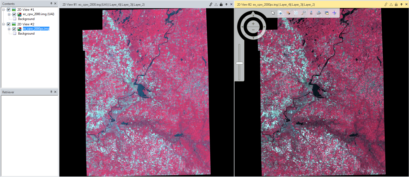 |
| (Fig. 3) Original image on the left and the pansharpened image on the right |
 |
| (Fig. 4) Zoomed in using the image sync feature to show the detail difference of pansharpening. |
Radiometric Enhancement Techniques
One application of radiometric enhancement techniques is to reduce the amount of haze from a satellite image has. Selecting Radiometric the Raster tab you will get a list of options. For the objective in this lab I selecting Haze Reduction tool from the previous tabs to complete the task.
Looking at the images side by side you will see the original image had a high concentration of haze or cloudiness in the south eastern corner of the image. Looking at the haze reduced image the haze is no longer visible on the image. In fact the color in the image is more vibrant.
 |
| (Fig. 5) Image prior to Haze Reduction on the left and after on the right. |
Google Earth Linking
Advancements in ERDAS Imagine 2011 allowed Google Earth Linking, a new feature previously not available to be introduced. ERDAS has kept this feature going in the 2015 version.
Google Earth linking allows the analysis to compare an image from Google Earth next to a satellite image for increased interpretation abilities. The first step in linking is to click on Google Earth under the main subheadings.
 |
| (Fig. 6) Location of the Connect to Google Earth button. |
After bringing in the Google Earth image you have the ability to sync and link the views together. When you zoom in to the original image the second viewer will zoom in to the same area on the Google Earth image. Utilizing Google Earth for interpretation purposes is called using an selective image interpolation key.
 |
| (Fig. 7) Image from ERDAS on the left and the synchronized image from Google Earth on the right. |
Resampling Satellite Images
The process of resampling changes the pixel size of the image. Within ERDAS you have the ability to resample up (increase) or down (decrease) in pixel size. To accomplish this task I use the Resample Pixel Size tool under the Raster and Spatial menu. Within this tool there is a number of different methods to achieve resampling. Using the Nearest Neighbors method I resampled the image from 30x30 meters to 15x15 meter pixel size. Examining a second method I utalizied Bilinear Interpolation method to resample the same image to 15x15 meters pixel size. The difference between the two different methods is visible when zoomed in on the images. If you look at (Fig. 8) you will notice actual pixel squares are visible in the left image (Nearest Neighbors method) along the edges of the blue areas. Comparing the same area in the image on the right (Bilinear Interpolation) you will notice the image edges are smoother. When you zoom into the image using the Bilinear Interpolation you can notice there are pixel squares in the image, they are just smaller than the Nearest Neighbors image.
 |
| (Fig. 8) Synchronized view of Nearest Neighbors (Left) and Bilinear Interpolation (right) resampling methods. |
Image Mosaicking
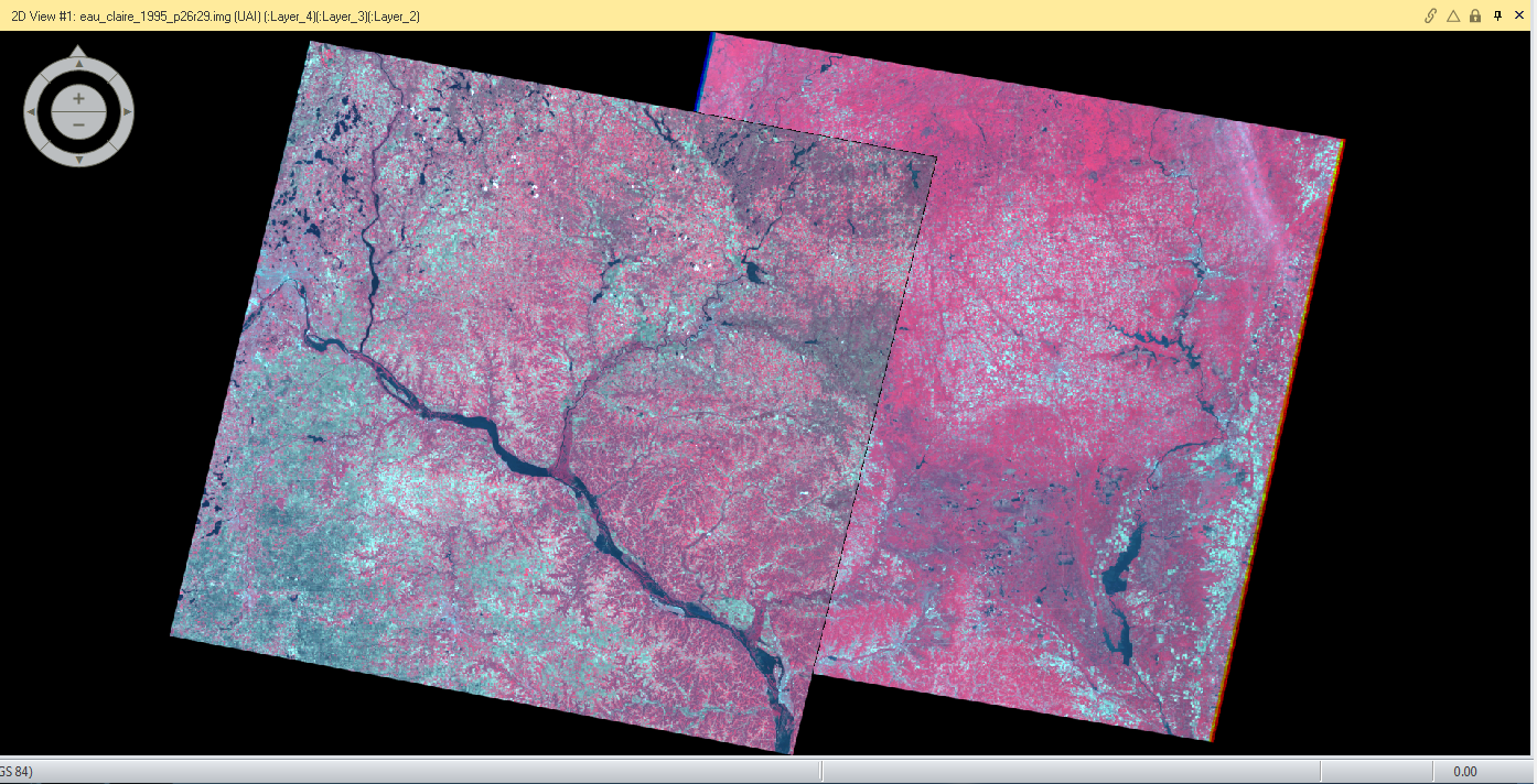
There are times in remote sensing where your study area extends beyond the spatial extent of one satellite image. Additionally, there are times when your study area covers an area which crosses two different satellite images. The process of combining 2 or more images together for interpretation is called Image Mosaicing.
ERDAS has a couple options for mosaicing. I will be exploring Mosaic Express and Mosaic Pro withing ERDAS Imagine. Mosaic Express is a simple and quick method to combine to images for basic visual interpretation. One should never do serious model analysis or interpretation of a Mosaic Express image.
For serious image analysis and interpretation one should use Mosaic Pro within ERDAS Imagine. Mosaic Pro gives you a host of options to assure your image will give you proper representation. However, to properly use the Mosaic Pro option, you must properly set all of the parameters to have the output file the way you want it. One of the key elements is to organize the images with the "best" (least amount of haze, clouds, and distortion) one on top.
For this section of the lab we used both of the options for mosaicing. I utilized the same images for both and after running the Mosaic tools I displayed them in separate views to show the difference in the methods.
 |
| (Fig. 9) Viewer window with both the images to be mosaicked together. |
 |
| (Fig. 10) Mosaic Express image (Left) and Mosaic Pro image (Right) |
Binary change detection (image differencing)
Section 1
Binary change is the change in pixels from one image to the next. For this part of the lab we will examine the change of band 4 between an image from 2011 and 1991 (Fig. 11).
 |
| (Fig. 11) 1991 image (left) 2011 image (right) |

Section 2
To visually display the areas which have changed between the two images I need to use a different approach. Utilizing Model Maker under the Toolbox menu, I developed a model to get rid of the negative values in the difference image I created in Section 1. Using an algorithm provided to me from Dr. Wilson (Fig. 13) I subtracted the 1991 image from the 2011 image and added the constant value.
 |
| (Fig. 13) Algorithm from Dr. Cyril Wilson. |
After running the model maker tool I had a histogram that was comprised of all positive values. Since I added the constant to avoid getting the negative numbers when I determine the change threshold I will have to use mean + (3*standard deviation) of the mean. After calculating the
change/no change threshold value, I created a Either or function definition. If the number was above the change threshold value then it would display a pixel and if it was not above then it would mask out the pixel. After running this model, I overlayed the results on an image of the study area for display purposes (Fig. 14).

Conclusion
This lab was a great introduction to some of the capabilities withing ERDAS Imagine, and techniques to properly interpret and analyze images. The tools and methods explored in this lab are used by remote sensing experts every day. I looked forward to using these newly found skills in future labs, exercises and career.
Sources
Images provide to me from Dr. Cyril Wilson were from Landsat 4 & 5 TM.