Remote Sensing Lab #6: Geometric correction

Goals and Background

The goal of this lab is to give us an introduction to a preprocessing method called geometric correction.  Geometric correction is required to properly align and locate an aerial image.  Aerial images are never perfectly inline due to a multitude of factors which alter the angles of the image.  Within this lab exercise we will explore and practice two different methods of geometric correction.

Rectification is the process of converting a data file coordinate to a different coordinate or grid style system known as a reference system.

1. Image-to-Map Rectification:  This form of geometric correction utilizes a map coordinate system to rectify/transform the image data pixel coordinates.

2. Image-to-Image Rectification:  This form of gemteric correction uses a previously corrected image of the same location to rectify/transform the image data pixel coordinates.

Methods

The first method I explored in the lab was Image-to-Map-Rectification.  For this exercise we used a USGS 7.5 minute digital raster graphic (DRG) covering a portion of Chicago, Illinois to geometrically correct a Landsat TM image of the same area (Fig.1).  I will be performing this task in Erdas Imagine 2015.

(Fig. 1) The USGS DRG is on the left and the uncorrected image of Chicago area is on the right

I will be utilizing the Control Points option under the Multispectral tab in Erdas to perform the geometric correction.  After opening the Control Points option I set the Geometric Model to Polynomial and used the first order polynomial equation per directions from my professor.  I also set the USGS DRG map as the reference image.

To correct the image I will be placing ground control points (GCP) on both maps in the same locations using the "Create GCP" tool within the correction window.  At this extent in (Fig. 1) it is hard to be super precise when placing GCP's so after they are placed you can zoom in and adjust them to have a more precise location.  When placing GCP's you want to use fixed locations like "T" intersections of roadways or permanent buildings which have been in the area for a long time.  It is not advisable to used features such as lakes or rivers as they change over time and their locations may be different from image to image.  The accuracy between my GCP points is automatically calculated by Erdas in Root Mean Square (RMS) error.  The industry standard in remote sensing is .5 RMS error or below.  For this first exercise I was only required to reach an RMS error of 2 since this was my first attempt of geometric correction.

I place four GCP's per my instructions in the general area requested by my professor (Fig. 2).  I zoomed in and continued to adjust the points till I was able to achieve a .2148 RMS error, well below the industry standard.  There was very minimal error in the image we corrected, so displaying the correction is very difficult.  In the next correction process you will be able to see and visible change from the original image to the corrected image.

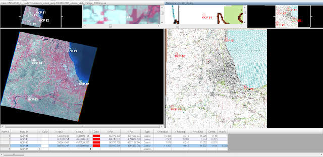
(Fig. 2)  First placement of the four GCP's for geometric correction.

(Fig.3) Zoomed in view while adjusting the GCP locations more precisely.

The second method of Image-to-Image Rectification was explored using two satellite images of Sierra Leone.  The process of Image-to-Image Rectification is exactly the same as the Image-to-Map method except you are utilizing an image which has been previously corrected as your reference.

The settings for the Control Point tool were all the same with the exception of changing from the first order polynomial to the third order polynomial.  This setting adjustment will require more GCP's to geometrically correct the image.  The additional GCP's will add to the precision of the correction.  I was instructed to place 12 GCP's on the image in specific locations provided to me by my professor.

(Fig. 4)  The two images displayed using the Swipe tool showing the error in the bottom (uncorrected) image.

After performing the same opperation as the previous image I adjusted all 12 of the GCP's until my RMS error was .1785.  I used bilinear interpolation to resample the image and export it as a new file.  The next step was to bring in the resampled image and compare it to the reference image to inspect the accuracy of my geometric correction.  The alignment was perfect as expected.  The corrected image appears hazy but a simple image correction operation in Erdas would remedy the issue.

(Fig. 4)  The corrected image (top) aligned with the reference image (bottom).

Results

This lab exercise gave me a basic understanding of geometric correction.  Having images which are geometrically correct is essential for proper and accurate analysis.  Geometric error may not always be visible to the human eye, however all images should be checked and then corrected for any errors before analysis is completed.   Locating good areas for GCP location is something which takes a bit of practice which was effectively translated in this lab.

Sources 

All images were acquired from the United States Geologic Survey (USGS).

Remote Sensing Lab #5: Lidar

Goals and Background

The goal of this lab is to obtain a basic understanding of Lidar data and processing.  In this lab we will be using Lidar point clouds in LAS file format to create various models of the earths surface.  Lidar has had a significantly growth in the remote sensing field, creating many jobs.  Understanding this information will give me an additional tool as my career advances.

Lidar is a active remote sensing system.  The system sends a laser pulse from an aircraft towards the ground and then a sensor mounted on the aircraft receives the return pulse from the ground (Left, Fig. 1).  From this data the system produces point cloud data.  From this data we are able to calculate location and elevation.  The return data is broken down into return heights (Right, Fig. 1). 

(Fig. 1) (Left) Depiction of Lidar system on an aircraft. (Right) Example of return levels of lidar. (https://ic.arc.losrios.edu/~veiszep/28fall2012/Fancher/G350_ZFancher.html)

Methods

The first section of the lab had us importing Lidar point cloud files into Erdas Imagine for a visual understanding (Fig. 2).  Additionally, we inspected the Tile Index to help located where specific tiles lie within the study area (Fig. 3).

(Fig. 2)  LAS point cloud files of a portion of Eau Claire County displayed in Erdas Imagine.

To gain better understanding of where the study area was, I opened the tile index in ArcMap.  The next step was to open the same LAS files from the first step in ArcMap.  The LAS files opened were only just a small portion of the full tile index (Fig. 2)  Next, I was able to calculate and inspect the statistics in the properties window.  Analyzing the statistics revealed the elevation (z-values) to be higher than the actual elevation of the study area (Fig. 4).  The elevation for the study area is just a little shy of 1000 ft, so the z-value of 1800 is an anomaly.  I will examine and determine why the z-value is so high later in this lab.

(Fig. 3) The tile index with the LAS files overlayed in ArcMap.

(Fig. 4) Statistics of the LAS dataset.

The majority of older Lidar data is delivered to the analysis without having a coordinate system defined in the dataset.  The information is available within the metadata but as the analyst I have to the define the coordinate systems before use.  Switching to the XY Coordiante System tab in the LAS Dataset Properties I defined the dataset to the appropriate projection for both the horizontal and the vertical coordinate system.

With the point cloud dataset open in ArcMap I examined the surface data in four different methods/conversion tools on the LAS Dataset Toolbar:  Elevation, Aspect, Slope, Contour.  I found the elevation to be the most useful for multiple forms of analysis.  Aspect, slope, and contour have there uses but are more limited.

(Fig.5) Point cloud data displayed in ArcMap.

The area is (Fig. 6) which appear to be a mountain is actually in the middle of the river.  This has to do with the interpolation method used to generate the display.  Inspecting (Fig. 4) you can see there is no real data within the river area.  The elevation to essentially just makes an educated guess as to the topology of the area.

(Fig. 6) The elevation conversion of the point cloud data in ArcMap.

I will be examining the first returns of the elevation point cloud image utilizing the LAS Dataset Profile View tool with in ArcMap.  Using the information from the statistics tables I zoomed in to the grid square with the highest elevation to attempt to locate the cause of the anomaly of the high elevation value.  After a little searching and the use of the 3D View I was able to locate the points with the profile view (Fig. 7).  My guess is the feature well above the majority of the points is some form of communication tower.

(Fig. 7) Profile view with in ArcMap of Lidar point cloud data.

One of the great aspects of Lidar is the ability to derive 3 dimensional images from the data.  These images have a multitude of uses.  For this lab I will be creating a digital surface model (DSM) with the first return data at a spectral resolution of 2 meters.  I will also be creating a digital terrain model (DTM) and a hillshade model of both the DSM and DTM.

Before creating the images I had to set the display parameters in ArcMap correctly.  I set the layer to display the points by elevation and only utilized the first returns.  Using LAS Dataset to Raster tool in ArcMap I set the specifications as follows: Value Field=Elevation, Cell Type=Maximum, Void Filling=Natural Neighbors, Cell Size= 6.56168 (approximately 2 meters).  The tool take a few minutes to run, but once it is done you have visual image of the elevation of the study area (Fig. 8).  The image leaves a little to be desired as far as visual clarity.  To enhance the detail of the image I will created a hillshade of the DSM (Fig. 9).

(Fig. 8)  DSM model created within ArcMap.

(Fig. 9) DSM model with hillshade enhancements.

Next using the same tool I will create a DTM or in a simpler term a "bare earth" raster image.  The image will display only the ground elevation and none of the buildings or trees.  This is a great tool to get a good understanding of the terrain when working in an area.

I set the filter to Ground returns and left the point elevation.  I used the LAS Dataset to Raster tool again with the same settings.  The result is an image of the same area from the DSM but without all the above surface features (Fig. 10)

(Fig. 10) DTM of the same study area as above.

The final transformation I conducted was to create a Intensity image based on the Lidar point cloud information.  The intensity image is collected in the first return.  Before running the tool I set the filter to first returns.  Using the LAS Dataset to Raster tool I left all of the settings the same as before except the Value Field which I changed to INTENSITY.  After the tool was complete the image was very dark and not very detailed or visable.  I could have adjusted the setting with in ArcMap to alter the view but a simpler method was to open the image in Erdas Imagine (Fig. 11).  Erdas enhances the display of the image on the fly.

(Fig. 11) Intensity image created in ArcMap, viewed in Erdas Imagine.

Results

I now have a solid base understanding of how Lidar works and the data which results.  The operations I preformed above are just the basics in the utilization of Lidar data.  To become proficient at Lidar one would have to take multiple classes to fully understand all of the process associated with production and use of the data.  I look forward to future exploration of Lidar processes.

Sources

Lidar point cloud and Tile Index obtained from Eau Claire County, 2013.
Eau Claire County Shapefile is from Mastering ArcGIS 6th Edition data by Margaret Price, 2014.